In this paper, we obtain convergence of a posteriori error indicator to 0 when the mesh size h goes to 0 for the finite element approximation of source-boundary control problems governed by a system of semi-linear elliptic equations. We give the upper and lower bound of a posteriori error, and convergency of a posteriori error indicator.
| Published in | Mathematics Letters (Volume 11, Issue 2) |
| DOI | 10.11648/j.ml.20251102.12 |
| Page(s) | 41-59 |
| Creative Commons |
This is an Open Access article, distributed under the terms of the Creative Commons Attribution 4.0 International License (http://creativecommons.org/licenses/by/4.0/), which permits unrestricted use, distribution and reproduction in any medium or format, provided the original work is properly cited. |
| Copyright |
Copyright © The Author(s), 2025. Published by Science Publishing Group |
Semi-linear Elliptic Equations, Source Control, A Posteriori Error Estimate
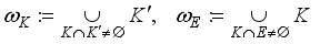
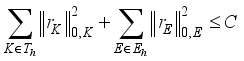
 is denoted as the form of sum with respect to elements of an indicator
  , i.e., as the form of infinite series when h goes to 0 unlike spectral method.
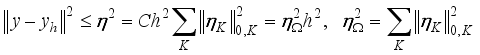
 denote the
  norm and inner product. We set
  ,
,  with
with  .We denote by
  or
or  the
the  norm and inner product, and by
  the
the  -norm and duality product between
  and
and  .
.  be a bounded convex polygonal domain in
  with boundary
  .
. 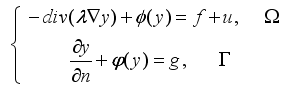 (1)
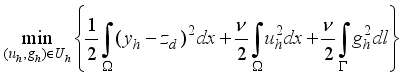
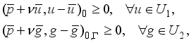
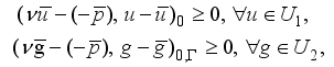
(1)  are to be controlled and the feasible sets are convex closed subsets of
  as follows.
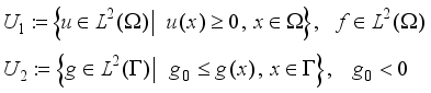
 .
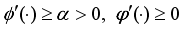
.  and they are strictly monotonic in

 (2)
(2)  is given,
 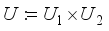 .
. 
 is a solution of (2).
  is a solution of Problem 1. There exists
  that satisfies:
 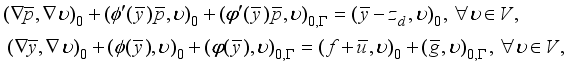 (3)
(3)  in the
  in the direction of
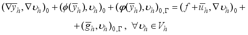
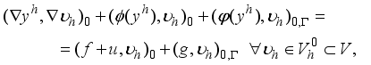
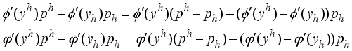
 satisfy the following equations, respectively.
 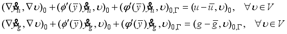 (4)
(4)  in the direction of
  are as follows:
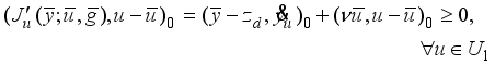
 of the following adjoint system.
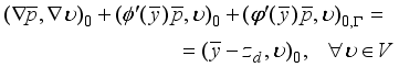
 .
.  in the second equation of (4) and
  in the adjoint system, and comparing them, we get
  .
. 
 into regular triangles
  and denote the diameter of a triangle
  by
by  , respectively. We set
  , let
, let  be the family of triangles,
  the set of all the sides of the triangles and denote finite element function space of
  as:
as: 
 denotes a polynomial space whose order is less or equal than one on element
  .
. 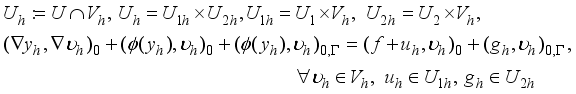 (5)
(5) 
 is the unique solution of(5).
  , which satisfies the following system (optimality system)
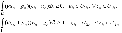
 (6)
(6) 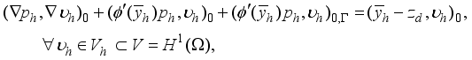 (7)
(7)  is the unique solution of (7).
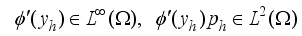
  :
:  denote an orthogonal projection operator. For
  , we have:
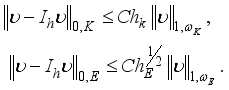

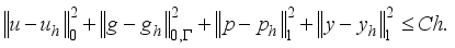
 is the solution of problem 1, then
  .
. 
 and
and 
 by assumption 1,
  from the smoothness of the solution of an elliptic equation and
  has a unique solution in.
 , the continuity of
  and
and  and the properties of operator
  , the assertion of the theorem holds.
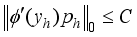
  is coercive with respect to
  ,
,  are bounded independent of
  . In the below equation satisfied by
 when considering the asumption 1, we get


 are norm equivalent constants of spaces
  and
and  is a constant independent of
  .
. 
 ,
,  .
. 
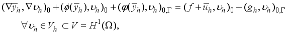
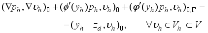
 satisfies the following system
 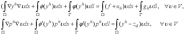 (8)
(8)  is a unique solution of the first expression of (5).
  (9)
(9)  is an arbitrary element in the neighborhood of
  .
. 

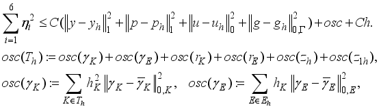
 .
. 
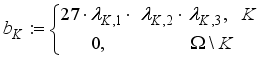
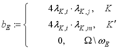
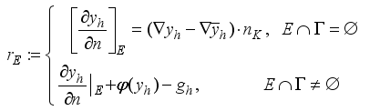
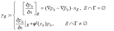
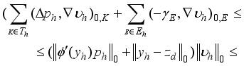
 are as follows.
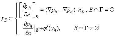
 is the jump value of the directional derivative in the common boundary
  of two elements
  .
. 
 is the jump value of the directional derivative in the common boundary
  of two elements
  .
. 
 are positive, seen in theorem 1.
 and 1) of lemma 2, we get
 .
. 
 ,
,  .
. 
 is a strictly monotonic constant of in assumption 1.
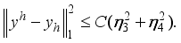
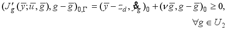
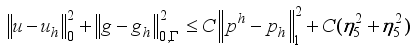
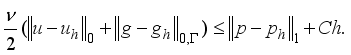
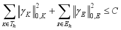
 are the solutions of (3) and (6), (7) respectively, then the following relation holds.
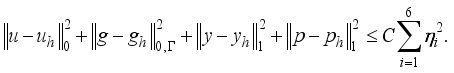
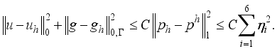 (10)
(10)  (11)
(11)  (12)
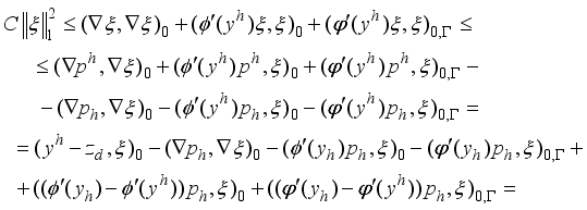
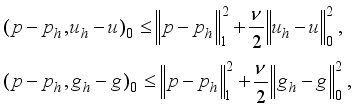
(12)  , setting a test function as
  and using the strong monotonicity of
  and the monotonicity of
  , we get
 .(13)
.(13)  , setting a test function as
  and considering assumption 1, we get
 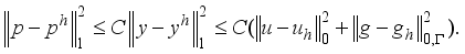 (14)
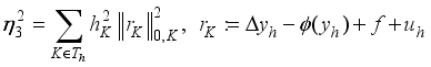
(14)  of element
  .
. 
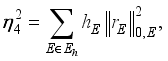
 is a common edge of elements
  .
. 
 and edge
  ,
,  have the following properties.
 .
. 


 .
. 


 .
. 


 .
. 

 .
. 

 .
. 
 .
. 

 .
. 

 . For convenience, we accept the following notation
  .
. 
 .
. 
 .
. 

 , we get the result of the theorem.
 is the solution of the following equation.
 is a constant independent of
  .
.  (15)
(15)  (16)
(16)  as
as  and fix
  .
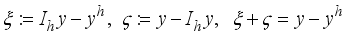
.  be a standard interpolation operator.
  and we define
  as
as 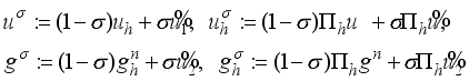 (17)
(17)  .
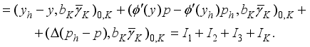
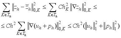
.  add together and put in order, then we get
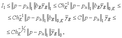
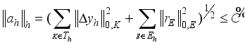
 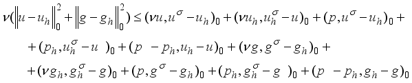 (18)
(18)  (19)
(19) 
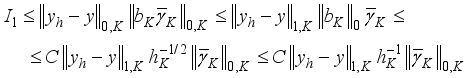
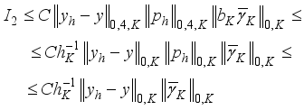
 and considering the boundedness (lemma 2) of finite element solutions independent of
  , we get the estimation.

 (20)
(20) 
 the different constants independent of
  .
. 
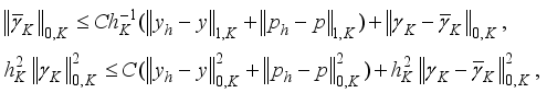
 . Taking into account the assumption 1, we get
 is positive seen in assumption 1.
 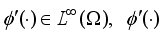 and 1) of lemma 2, we get
  (21)
(21)  .
.  .
. 
 (22)
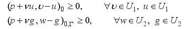
(22)  satisfy, it holds that
 and consider the strong monotonicity of
  and monotonicity of
  , then we get
  (23)
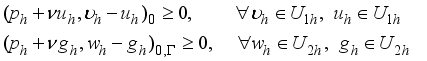
(23)  satisfy, we get
 ,
,  and set a test function as
 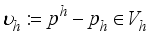 , we get the following expression
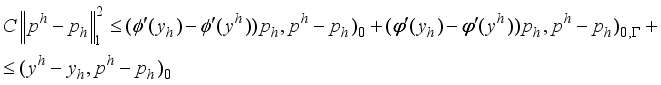
 is positive seen in assumption 1.
 (24)
(24)  (25).
(25). 
 to satisfy
  . Then it holds that
  (26)
(26)  .
.  , it holds that
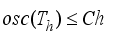
 all the constants independent of
  .)
.)  (
(  is independent of
  ). Here,
  are defined in lemma 5 to be
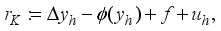
 (27)
(27)  is a constant independent of
  .
.  and by assumption 1,

 .
.  as
as 
 In
In  , we think of a functional
  .
.  ,
,  is a bounded linear functional in
  and by Riesz’ representation theorem, there exists a unique element
  ,
,  such that
  .
.  (28)
(28)  (
(  is independent of
  ), we get
 .
.  (
(  is a constant independent of
  ). Here,
  are defined in lemma 5 to be as follows.
 , (
, (  are independent of
  )
)  , introducing a functional
 such that
  and
and  . Therefore, it holds that
  ,
, 
 (29)
(29) 
 , we get.
 .
.  .
. 
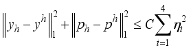
 be the solutions of (5) and (6), (7) respectively. When
  , the following convergence result about a posteriori error indicator holds.
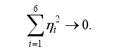
 . Using theorem 4 and lemma 8, the result follows from theorem 3.
 FEM | Finite Element Method |
| [1] | Wei Gong et al., Adaptive finite element method for parabolic equations with Dirac measure, Comput. Methods in Applied Mechanics and engineerig, 328(2018) 217-241. |
| [2] | Chunjia Bi et al., Two grid finite element method and it’s a posteriori error Estimates for a non-monotone quasi-linear elliptic problem under minimal regularity of data, Computers and Mathematics with Applications, 76(2018) 98-112. |
| [3] | Chuanjun Chen et al., A posteriori error Estimates of two grid finite volume element method for non-linear elliptic problem, Computers and Mathematics with Applications, 75(2018) 1756-1766. |
| [4] | Xingyang Ye, Chanju Xu, A Posteriori error estimates for the fractional optimal control problems, Journal of Inequalities and Applications, 141(2015), 1-13. |
| [5] | Lin Li et al., A posteriori error Estimates of spectral method for non-linear parabolic optimal control problem, Journal of inequalities and applications, 138(2018) 1-23. |
| [6] | E. Casas et al., Error Estimates for the numerical approximation of Dirichlet boundary control for semilinear elliptic equations, SIAM J. Control Optim., 45(2006) 1586-1611. |
| [7] | D. Y. Shi, H. J. Yang, Superconvergence analysis of finite element method for time-fractional thermistor problem, Appl. Math. Comput., 323 (2018) 31-42. |
| [8] | D. Y. Shi, H. J. Yang, Superconvergence analysis of nonconforming FEM fornonlinear time-dependent thermistor problem, Appl. Math. and Compu., 347 (2019) 210-224. |
| [9] | Y. Chen, L. Chen, X. Zhang, Two-grid method for nonlinear parabolic equations by expande mixed finite element methods, Numer. Methods Part. Diff. Equ., 29(2013) 1238-1256. |
| [10] | Meyer C., Error estimates for the finite element approximation of an elliptic control problem with pointwise state and control constraints, Control and Cybern., 37(1), 51-83 (2008). |
| [11] | Wollner W., A posteriori error estimates for a finite element distretization of Interior point methods for an elliptic optimization problem with state constraints, Numer. Math. Vol. 120, No. 4, 133-159 (2012). |
| [12] | A. Rosch, D. Wachsmuth, A posteriori error estimates for optimal control problems with state and control constraints, Numerische Mathematik, Vol. 120, No. 4, 733-762 (2012). |
| [13] | O. Benedix, B. Vexler, A posteriori error estimation and adaptivity for elliptic optimal control problems with state constraints, Comput. Optim. Appl., 44(1), 3-25 (2009). |
| [14] | Dib S., Girault V., Hecht F. and Sayah T., A posteriori error estimates for Darcy’s problem coupled with the heat equation, ESAIM Mathematical Modelling and Numerical Analysis, |
| [15] | A. Allenes, E. Otarola, R. Rankin. A posteriori error estimation for a PDE constrained optimization problem involving the generalized Oceen equations, SIAM J. Sci. Comput., Vol. 40, No. 4, A2200-A2233, 2018. |
| [16] | Natalia Kopteva. Error analysis of the L1 method on graded and uniform meshes for a fractional-derivative problem in two and three dimensions. Math. Comp., 88(319): 2135-2155, 2019. |
| [17] | Xiangcheng Zheng and Hong Wang. Optimal-order error estimates finit element approximations to variable-order time-fractional diffusion equations without regularity assumptions of the true solutions. IMA J. Numer. Anal., 41(2): 1522-1545, 2021. |
| [18] | Natalia Kopteva. Pointwise-in-time a posteriori error control for time-fractional parabolic equations. Appl. Math. Lett., 123: Paper No. 107515, 8, 2022. |
APA Style
Kim, C. I., Kang, J. H., Sok, G. C. (2025). A Posteriori Error Estimates and Convergence of Error Indicator by FEM for a Semi-linear Elliptic Source-boundary Control Problem. Mathematics Letters, 11(2), 41-59. https://doi.org/10.11648/j.ml.20251102.12
ACS Style
Kim, C. I.; Kang, J. H.; Sok, G. C. A Posteriori Error Estimates and Convergence of Error Indicator by FEM for a Semi-linear Elliptic Source-boundary Control Problem. Math. Lett. 2025, 11(2), 41-59. doi: 10.11648/j.ml.20251102.12
AMA Style
Kim CI, Kang JH, Sok GC. A Posteriori Error Estimates and Convergence of Error Indicator by FEM for a Semi-linear Elliptic Source-boundary Control Problem. Math Lett. 2025;11(2):41-59. doi: 10.11648/j.ml.20251102.12
@article{10.11648/j.ml.20251102.12,
  author = {Chang Il Kim and Jong Hyok Kang and Gi Chol Sok},
  title = {A Posteriori Error Estimates and Convergence of Error Indicator by FEM for a Semi-linear Elliptic Source-boundary Control Problem
},
  journal = {Mathematics Letters},
  volume = {11},
  number = {2},
  pages = {41-59},
  doi = {10.11648/j.ml.20251102.12},
  url = {https://doi.org/10.11648/j.ml.20251102.12},
  eprint = {https://article.sciencepublishinggroup.com/pdf/10.11648.j.ml.20251102.12},
  abstract = {In this paper, we obtain convergence of a posteriori error indicator to 0 when the mesh size h goes to 0 for the finite element approximation of source-boundary control problems governed by a system of semi-linear elliptic equations. We give the upper and lower bound of a posteriori error, and convergency of a posteriori error indicator.
},
 year = {2025}
}
TY  - JOUR
T1  - A Posteriori Error Estimates and Convergence of Error Indicator by FEM for a Semi-linear Elliptic Source-boundary Control Problem

AU  - Chang Il Kim
AU  - Jong Hyok Kang
AU  - Gi Chol Sok
Y1  - 2025/09/03
PY  - 2025
N1  - https://doi.org/10.11648/j.ml.20251102.12
DO  - 10.11648/j.ml.20251102.12
T2  - Mathematics Letters
JF  - Mathematics Letters
JO  - Mathematics Letters
SP  - 41
EP  - 59
PB  - Science Publishing Group
SN  - 2575-5056
UR  - https://doi.org/10.11648/j.ml.20251102.12
AB  - In this paper, we obtain convergence of a posteriori error indicator to 0 when the mesh size h goes to 0 for the finite element approximation of source-boundary control problems governed by a system of semi-linear elliptic equations. We give the upper and lower bound of a posteriori error, and convergency of a posteriori error indicator.

VL  - 11
IS  - 2
ER  -
Department of Mathematics, University of Science, Pyongyang, DPR Korea
Department of Mathematics, University of Science, Pyongyang, DPR Korea
Department of Mathematics, University of Science, Pyongyang, DPR Korea


 of (
of ( .
.  are unique solutions of (
 .
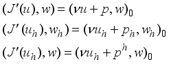
.  denote Gateaux differential of the solution of (
 at
at  in the direction of
  ,
,  in the first equation of (
 in the adjoint system, and comparing them, we get
  of (
of ( .
.  is a function defined in (
 is a constant independent of
  and
and  .
.  be the solutions of (
 is a constant independent of
  .
.